

Okay, you finished your first high throughput screening campaign, and now you need to decide which compounds are standing out for the validation/secondary assays. There are two strategies to select hits. You can either rank the samples based on their effect size in the assay and pick top performers or you can pick samples that meet the pre-set threshold. In either case, the goal is to maximize true-positive rates while minimizing false-negative rates (FNRs) and/or false-positive rates (FPRs). FP means wasting valuable resources in the secondary assay for inactive compounds (false discoveries), and FN means you might miss some valuable candidates in the primary round. Here, I will discuss a few common strategies/methods to identify true hits in primary HTS data while minimizing FNR and FPR.
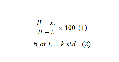
The first factor that affects the hit selection strategy is whether there are replicates for each compound or not. Because that indicates if we can calculate (and utilize) data variabilities on a sample basis or if we need to assume a sort of distribution. In most primary screening scenarios, and our focus here, there is only one copy for each compound in the screening pool. As a result, in screening without replicates, we rely on the strong assumption of the normal distribution for data variabilities. The second important factor is if we have controls (either one or both negative and positive). The benefit of controls-based methods is that they are straightforward to calculate, and can deal with systematic sources of HTS variability, assuming controls are affected similarly to samples. They can also be used to normalize the data across multiple runs/plates if needed. The following two formulas are some common approaches for hits selection if having controls. The first formula is useful if you want to rank samples and then pick top performers. This is a preferred method for screens with strong control where H and L are the average of High and Low controls. The second is used to test whether a compound has effects strong enough to reach a pre-set level by comparing it to the control value where “std” is the standard deviation of controls and K is an arbitrary multiplier. By changing k, you can make the selection criteria more or less stringer. K =3 is a reasonable choice if the normal distribution is assumed which translates to approximately 95% confidence level.
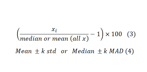
If there is no control in the screening, we can use the samples, themselves, as controls. “This may seem to be a contradiction, but in reality majority of samples in screening are not active and can serve as vehicle control”1. Formula 3 and 4 are counterparts for Formula 1 and 2 in case there is no control in the test. Substituting the mean with median and Standard Deviation (STD) with the Mean Absolute Deviation (MAD) helps with dealing with outliers and controlling false positive discovery rates. However, MAD gives equal weight to all deviations from the mean, regardless of their magnitude. This means that outliers or extreme values in the dataset have the same impact as any other data point. This can translate to higher FNR. Therefore the choice between the two depends on the distributional properties of the dataset.
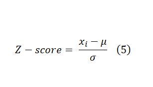
These formulas are easy to calculate and interpret. However, they fail to capture data variations and plate-to-plate or other locational biases. As a result, several statistical scoring methods have been developed to address these issues. Probably, the most widely known statistical scoring method in HTS is the Z-score (this is different from Z-factor). It is computed on a plate-by-plate basis, and it is calculated by Formula 5 below. Where μ and σ are the mean and standard deviation of all samples, respectively. You can use the Z-score as a cut-off which in this case ±3 is the common choice if you can assume normal distribution of data across the plate. Alternatively, you can use Z-score values to rank samples, and pick a fixed percentage of the most extreme samples.
Z-score can handle both multiplicative and additive offsets as it has the average on the numerator and standard deviation on the denominator. This is an important feature when processing and analyzing compounds across multiple plates (experimental unit). However, the Z-score still fails to handle positional effects (such as edge, row, and column effects). Its performance is also susceptible to extreme outliers as average and standard deviation are not affected by extreme values proportionally. This can be alleviated by using median and MAD instead. However, they also have their shortcomings. Another strategy is to use B-Score (for “better” score) which might offer better performance than Z-score. The B-score calculation is similar to the Z-score in that they are both the ratio of an adjusted raw value in the numerator to a measure of variability in the denominator. However, both the adjustment and measure of variability are more extensive. These adjustments make the B-score more resistant to positional effects (column and row) and outliers. It also enables combining (normalizing) data over all plates in the screening which might further reduce both false positive and false negative rates. On the other hand, B-Score calculation is more computationally demanding compared to Z-Score which requires specialized statistical software. Check Reference 1 for the full discussion on the B-Score calculations and applications.
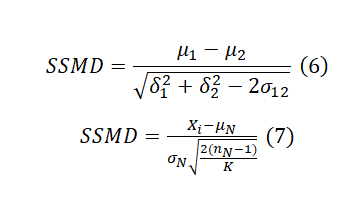
A more recent statistical scoring method is the strictly standardized mean difference (SSMD) which was originally introduced for quality control and hit selection in RNAi HTS assays. SSMD can be used to evaluate the differentiation between a positive control and a negative control in HTS assays (QC) or for sample ranking. The SSMD formula typically involves the means, standard deviations, and correlation coefficients between the groups being compared. The standard formula assumes the presence of replicates (Formula 6). In a primary screen without replicates, it can be rewritten as formula 7. Check SSMD Wikipedia for full annotation of each parameter.
As seen in Formula 6, SSMD standardizes the mean difference by dividing it by an estimate of the pooled standard deviation. This standardization process results in a dimensionless quantity that is not influenced by the scale of the original measurements. This makes the SSMD less sensitive to variations in scale and distribution. However, in cases without replicates, SSMD, as well as Z-score and B-Score, relies on the assumption that every compound has the same variability as the reference in that plate. In addition, we may get a large SSMD value when the standard deviation is very small, even if the mean (effect size) is small. Moreover, the SSMD value itself may be less intuitive to interpret compared to other effect size measures. Table 1 serves as a guideline for using the SSMD value for sample classification.
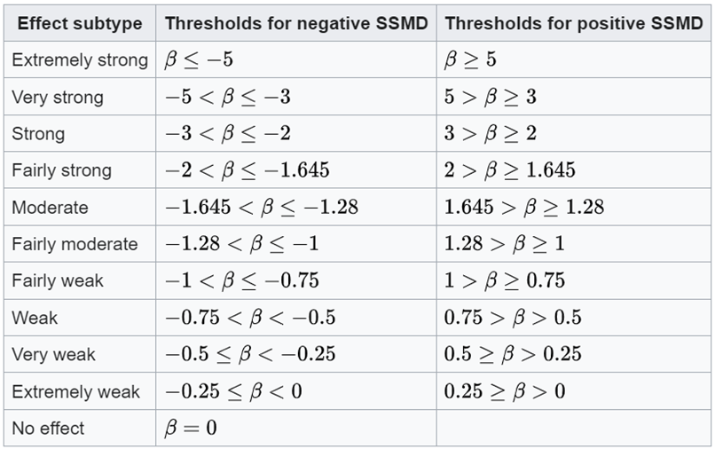
Table 1. SSMD to classify effects are shown based on the population value of SSMD. From Wikipedia
For most HTS cases, the common practice is to combine a statistical scoring method (such as SSMD, B-score, and Z-score) with a controls-based measure (such as average fold change), and then use another scoring method for backup and examination. As such, the dual-flashlight plot can be very useful to visualize and interpret the results. In a dual-flashlight plot, we plot a statistical scoring system (such as SSMD or p-value) versus an effect size measure (such as average log fold-change or average percent inhibition/activation) on the y- and x-axes, respectively, for all compounds investigated in an experiment (figure 1 below). I might have a separate post on the dual-flashlight plot in the future.
In summary, there is a growing list of statistical methods (and hence software) to analyze HTS data and to select hits. Each method has its pros and cons. When selecting a method, it is critical to understand its underlying assumption and the experimental setup such as the presence and quality of controls, replicates, and the nature of screening compounds (small molecules, proteins, RNAi …). A method that works perfectly for small molecule library screening in which strong controls usually exist might fail for screening proteins and RNAi which normally offers a narrower separation window. I highly recommend checking relevant literature to design your HTS data analysis strategy before starting the HTS campaign. It would be squandering to troubleshoot once hits are moved to the secondary assay stage.
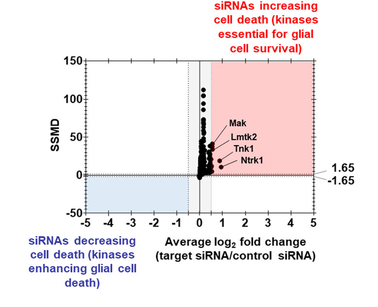
Figure 2. Example of a Dual-flashlight plot where strictly standardized mean difference is plotted versus fold change (log 2 scale) in the cytotoxicity assay. The figure is From here DOI:10.26508/lsa.202201605
This post was just an introduction to his selection in HTS. There will be more in-depth HTS data analysis posts here so subscribe to our newsletter now! If there is a topic that you would like to see here or have a question, please drop us a line at hello@assay.dev
References:
https://www.sciencedirect.com/science/article/pii/S2472630322002345
https://www.sciencedirect.com/science/article/pii/S0888754307000079